
Introduction
Basic Foundations in Translational Biomedical Informatics
Overview
The objective is to introduce individuals with strong backgrounds in biological and/or medicine with the foundations, basic principles, and core concepts in scripting and computing that are necessary in biomedical informatics. The abbreviated program will introduce concepts in data-science, command-line, scripting through Python and R. Upon successful completion of this abbreviated program, individuals will be able to: interface with the command line; create basic scripts in Python and R; and understand project management principles with strong underpinnings in data science. These introductory skills will serve as a foundational framework for individuals to build on in future courses or programs in biomedical data science.
- Data Basic Principles.
- Python Starter Kit.
- Data Science & Management Broad Principles.
- Command-Line & BASH.
Learning Environment
The goal is to learn through (1) written text within short-vignettes introducing major concepts, (2) screen-casts of the same or related content, (3) and through an interactive environment via Jupyter.
Written Content
Content and exercise are first provided as written HTML, viewable on any web-browser by clicking on any of the above links. Controlled vocabulary or terms or highlighted, external sources are hyperlinked, code to use within Jupyter is shown boxed:
data=5
print("data is ",data)
The output is shown in gray boxes:
data is 5
Screencasts
Screencasts are available reviewing the written content and working within the Jupyter Labs/Notebooks.
Jupyter Labs/Notebooks
These modules do not require you have a Linux/Unix based computer or have certain programs installed. All learning is done within browsers that run an environment where you can run Python, R, Command-line, and others: Jupyter Labs and Notebooks.
Jupyter Labs and Notebooks
Jupyter Labs is available at https://jupyter.org/try &
JupyterLab and Notebooks
JupyterLab and Jupyter Notebooks are a graphic interface for developing and writing Python code – and can be used for many other languages such as R, scala etc. A notebook usually means a single analysis or collection of scripts/code. The JupyterLab is a place for storing and managing many Notebooks. 
Using Browser-based Jupyter Notebook
You are welcome to install Jupyter on your computer, but we will generally just presume the Browser based version, which is here. 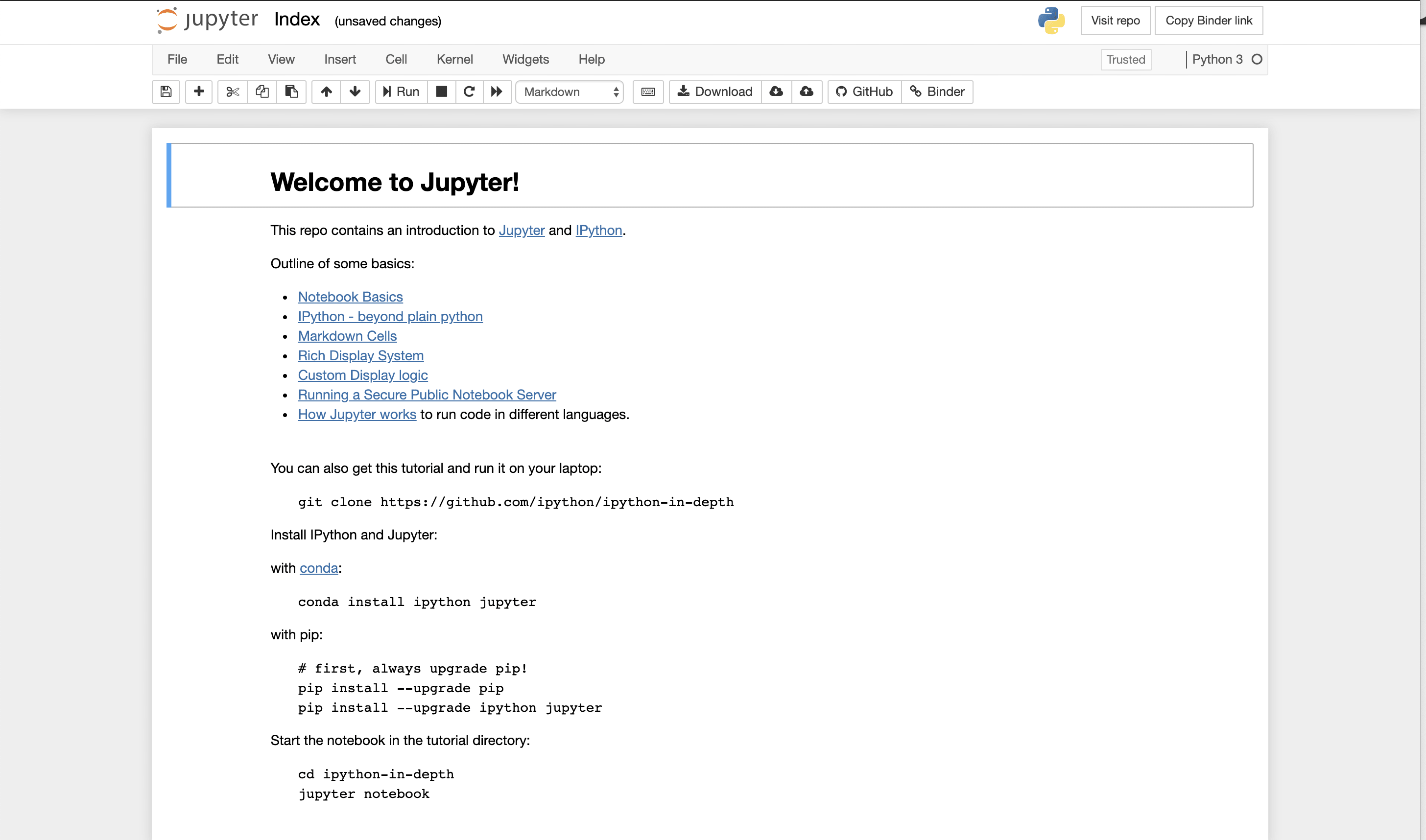
More Advanced Jupyter Lab!
Jupyter Lab provides more functionality and eventually is where you want to go. In many parts of the tutorial, we just use the notebook. However, if you want full functionality and saving, you do want to move to installing locally Jupyter Lab. There is a version that can be run within your browser. https://jupyter.org/try A snapshot is shown below. You can see in this view, you can see all files, you can edit and create what are called markdowns in the middle frame, and you have rendered markdowns in the right frame. We have discussed markdowns before, but basically they are a way of putting code and text together in a way that looks like a web page. 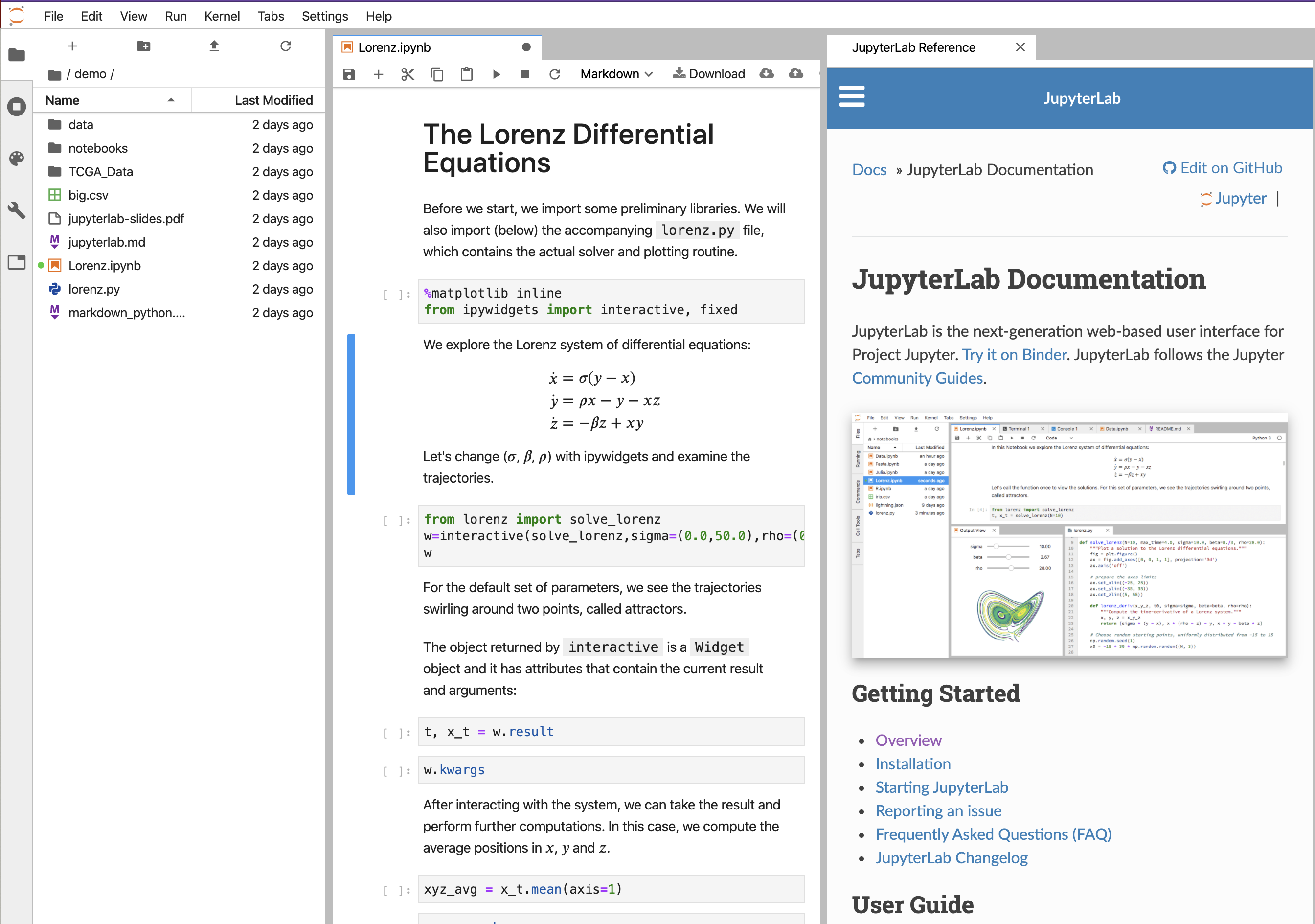 The code is run in cells by pressing the forward arrow after clicking on the cell.
You can see there are a lot of different types of files that can be created, and we discuss these in other modules. For this exercise, we largely just focus on the notebook 
Markdowns
Markdown is is a lightweight markup language that is plain text formatted, but is rendered to look like a web-page. It has a way of creating code-blocks. For example on the left we see Markdown. On the right we see the rendered view that could be published 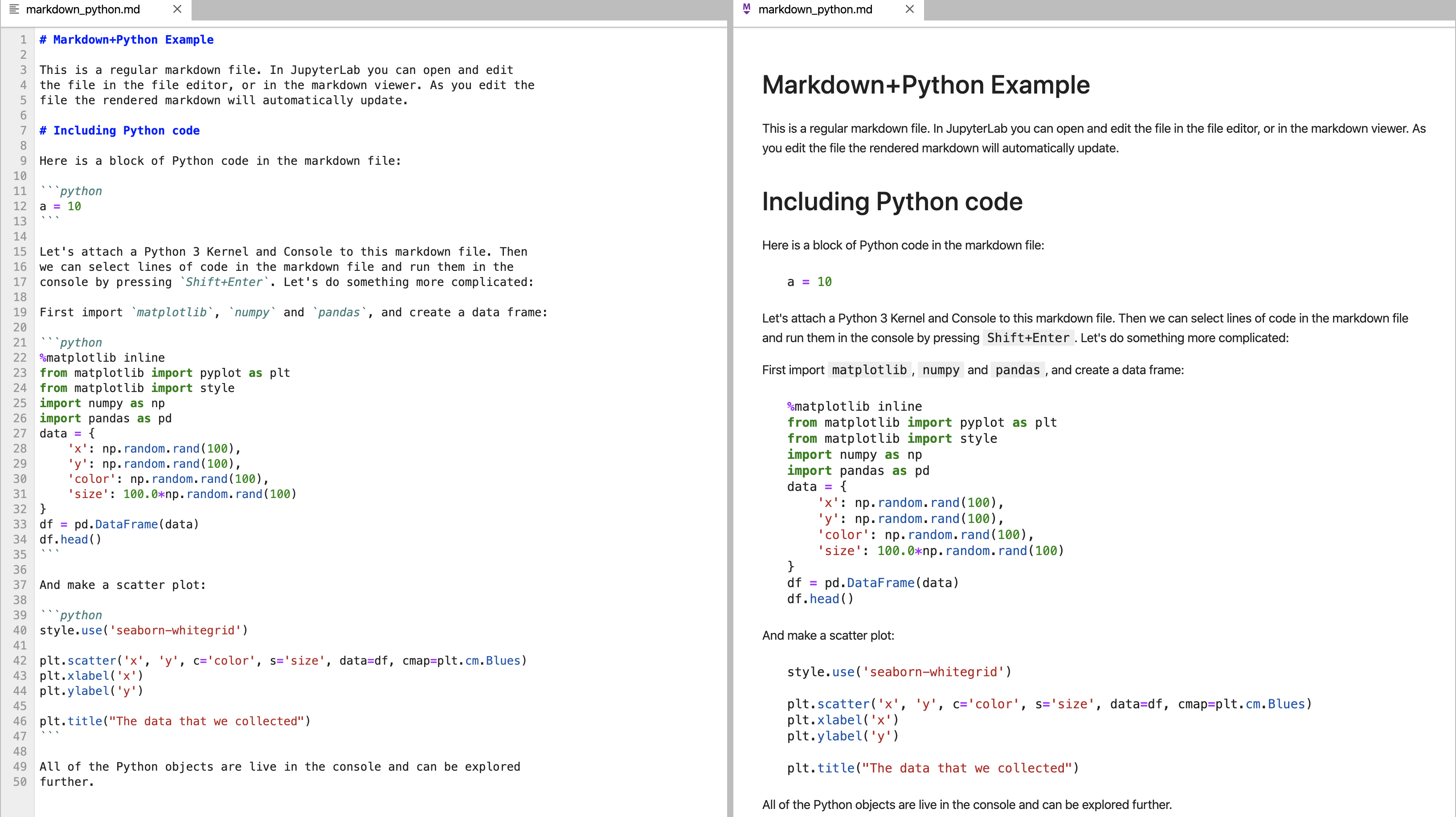
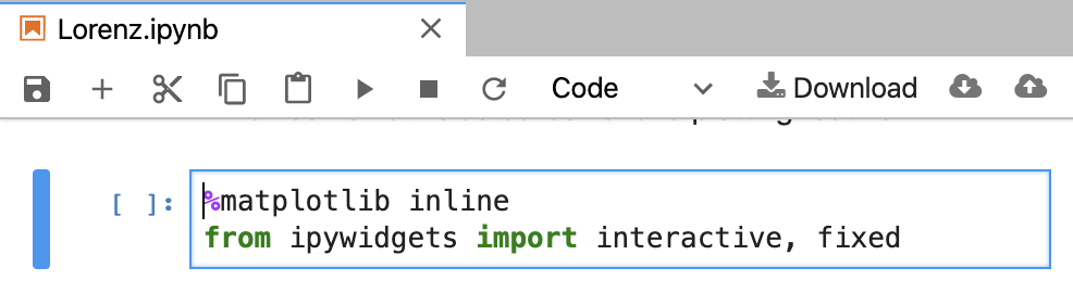
Code blocks are magical cells – creating interactive computing.
Now those code blocks are a bit magical in Jupyter lab as you’ll see. You’ll be edit and run them, seeing the results in a live interactive view. These types of markdowns that expect to be run and create a reproducible analysis are actually notebooks, and in Juptyer labs they end in .pynb. Notice that I can actually hit play or ‘run’ and see code by analyzed. 
We only scratch the surface.
There is quite a bit to learn, and to make the materials accessible, we only touch the surface. I encourage you to learn more about Jupyter Labs, Notebooks, and so forth. Its an amazing data science vehicle – and also a great learning tool.
Resources to Learn Outside of these Modules
Learning Flavors of Unix and Command-line
UNIX is an operating system around in the 60s and broadly refers to a set of programs that all work the same way at the command-line. They have the same feel. They have the same philosophy of design. Ok, its a specific operating system owned by AT&T, however, these days it refers to a program that all follow a common framework. There are many types of Unix – MacOSX, Linux, and Solaris where each of those is essentially different sets of codes owned by different companies or groups to get the common Unix common framework. MacOSX is owned and developed by Apple. Solaris is owned by Sun and Oracle. Linux is open-source and built from a community led by Linus Torvalds, and was meant to work on x86 PCs. The x86 refers to a type of CPU architecture used across most personal computers today (both Mac and PC). If I log into a Unix machine in 1980, 1990, 2000, 2010, 2017 – it will often feel and work the same.
- Kenneth Bradnam’s Command line Bootcamp (http://rik.smith-unna.com/command_line_bootcamp). Free one-page resource.
- Lynda.com
- Various modules dependent on need
- Code Academy (https://www.codecademy.com/). An excellent resource for learning without an account. Evaluated resources include Learn the Command-line, Website building, and Git. Can be tested for free, or utilizes a $19.95/mo fee
- Ryan’s tutorial (https://ryanstutorials.net/bash-scripting-tutorial/). Quick and easy w/ good instruction.
R
R is a scripting language enabled and expanded by RStudio. There is the base environment and the R-Studio environment which enables a graphical user interface (GUI) for editing and building reproducible analysis.
- Introduction to R by Thomas Girke.(https://girke.bioinformatics.ucr.edu/manuals/mydoc/mydoc_Rbasics_1.html)
- R & Bioconductor Manual by Thomas Girke UC Riverside (http://manuals.bioinformatics.ucr.edu/home/R_BioCondManual)
- Little Book of R for Bioinformatics (https://a-little-book-of-r-for-bioinformatics.readthedocs.io/). Free excellent book for pure R.
- DataCamp (https://www.datacamp.com/courses/free-introduction-to-r). Introductory tool for learning R. First few chapters are free, though it costs typically $25 per month
- R Basics Cheatsheet. Simple 1 page cheatsheet for basic R functions
- R Importing Data Cheatsheets. Simple 1 page cheatsheet for importing data into R.
- Transforming and manipulating data. Simple cheatsheets for manipulating data with dplyr.
- Top 50 ggplot2 Visualizations. (http://r-statistics.co/Top50-Ggplot2-Visualizations-MasterList-R-Code.html)
- FreeCodeCamp (2hr). Popular R video for learning R.
-
Lynda.com. Free for USC faculty , staff and students.
- Learning R (2hr 51min)
- R statistics (5h 59m)
- R for Data Science (7h 16m)
- Data Wranging in R (4 h 12 m
- Data Visualization in R with ggplot2
Exercises
Exercise 1: Joining Data
Analyzing & Interpreting Data
Exercise 2: Analyzing & Interpreting Data w/ Wordcloud
Visualizing Data