Biostatistics or biometrics is one of the single most important courses one can take – and is a foundation of much of bioinformatics.  In this section, we provide a review of some of the major concepts as a refresher – or to insure that you have some introduction to some major concepts.

Example Datasets

For this set of examples, we will have folks download a tar.gz which is a frequent way data is concatenated and compressed.

https://www.bioinform.io/site/datasets1.csv.tar.gz

wget http://itg.usc.edu/site/datasets1.csv.tar.gz
tar -xvf datasets1.csv.tar.gz
cd trgn510/

This yields the files below

trgn510/expression_results.csv
trgn510/kg.genotypes.csv
trgn510/kg.poplist.csv
trgn510/sample_info.csv

where expression_results.csv is the results of an expression study for multiple samples across multiple genes, and the description of the samples is sample_info.csv

We are also going to use `kg.genotypes.csv which is a file of genotypes recoded such that each individual at a specific position either matches the reference on both their maternal and paternal allele, is heterozygote, or homozygous for the alternative allele, encoded as 0, 0.5, and 1.  We also have information about the samples.

Mean

Variance / Standard Deviation

 Variance is the expectation of the squared deviation of a random variable from its mean. Variance is the expectation of the squared deviation of a random variable from its mean.

In R we can look at a summary(samples)

    patient        visit        reads                RIN          PF_BASES         PCT_RIBOSOMAL_BASES
 Min.   : 81.0   END  :48   Min.   : 14536426   Min.   :5.90   Min.   :1.181e+09   Min.   :0.008457   
 1st Qu.:705.0   Start:45   1st Qu.: 37903440   1st Qu.:7.90   1st Qu.:3.079e+09   1st Qu.:0.037450   
 Median :767.0              Median : 68197068   Median :8.40   Median :4.180e+09   Median :0.061019   
 Mean   :707.6              Mean   : 86575295   Mean   :8.26   Mean   :9.664e+09   Mean   :0.075703   
 3rd Qu.:807.0              3rd Qu.: 98329398   3rd Qu.:8.80   3rd Qu.:1.315e+10   3rd Qu.:0.085889   
 Max.   :917.0              Max.   :307503559   Max.   :9.90   Max.   :4.490e+10   Max.   :0.386714   
 PCT_CODING_BASES  PCT_UTR_BASES     PCT_INTRONIC_BASES PCT_INTERGENIC_BASES PCT_USABLE_BASES Kit   
 Min.   :0.03629   Min.   :0.06977   Min.   :0.2040     Min.   :0.03522      Min.   :0.0956   A:45  
 1st Qu.:0.13397   1st Qu.:0.22953   1st Qu.:0.3772     1st Qu.:0.05473      1st Qu.:0.3526   B:24  
 Median :0.14357   Median :0.28451   Median :0.4110     Median :0.07076      Median :0.4141   C:24  
 Mean   :0.14201   Mean   :0.28184   Mean   :0.4124     Mean   :0.08862      Mean   :0.4070         
 3rd Qu.:0.15689   3rd Qu.:0.31826   3rd Qu.:0.4581     3rd Qu.:0.08882      3rd Qu.:0.4593         
 Max.   :0.19701   Max.   :0.47429   Max.   :0.5784     Max.   :0.41524      Max.   :0.6118

Probability

Probability is the likelihood of something occurring.   If I role a 6-sided dice, I have a 1 in 6 chance of getting a 1. If I flip a two-side coin, I have a 50% chance of a head.  If I flip a 2 sided coin 50 times, what is the probability that I get 75 or more heads? We often write probability as:

p(X=4)=16.6%

that is the probability of getting a 4 is 16.6%

Probability Distributions

A joint probability distribution is a description of all the possibilities and the probability that they will occur.  If I role a six sided dice, I have an equal probability (16.6%) of getting a 1, as is the case for a 2,3,4,5,6.  Its often characterized by a Probability Mass Function (PMF) which provides the probability of each event. If I role a six sided dice, what is the probability that I get a 7?

Another key term is the Cumulative Probability Function (CMF), which is the sum that event or lower will have occurred.

There are a few probability distributions we care a lot about in bioinformatics.  The normal distribution (or Gaussian) and binomial distribution (binary events, such as a coin toss). Normal distributions are common in biology – but cannot always be presumed.  A normal distribution is famously represented as a bell curve.

 

a_mean <- aggregate(samples$reads, by=list(samples$Kit), FUN=mean) 

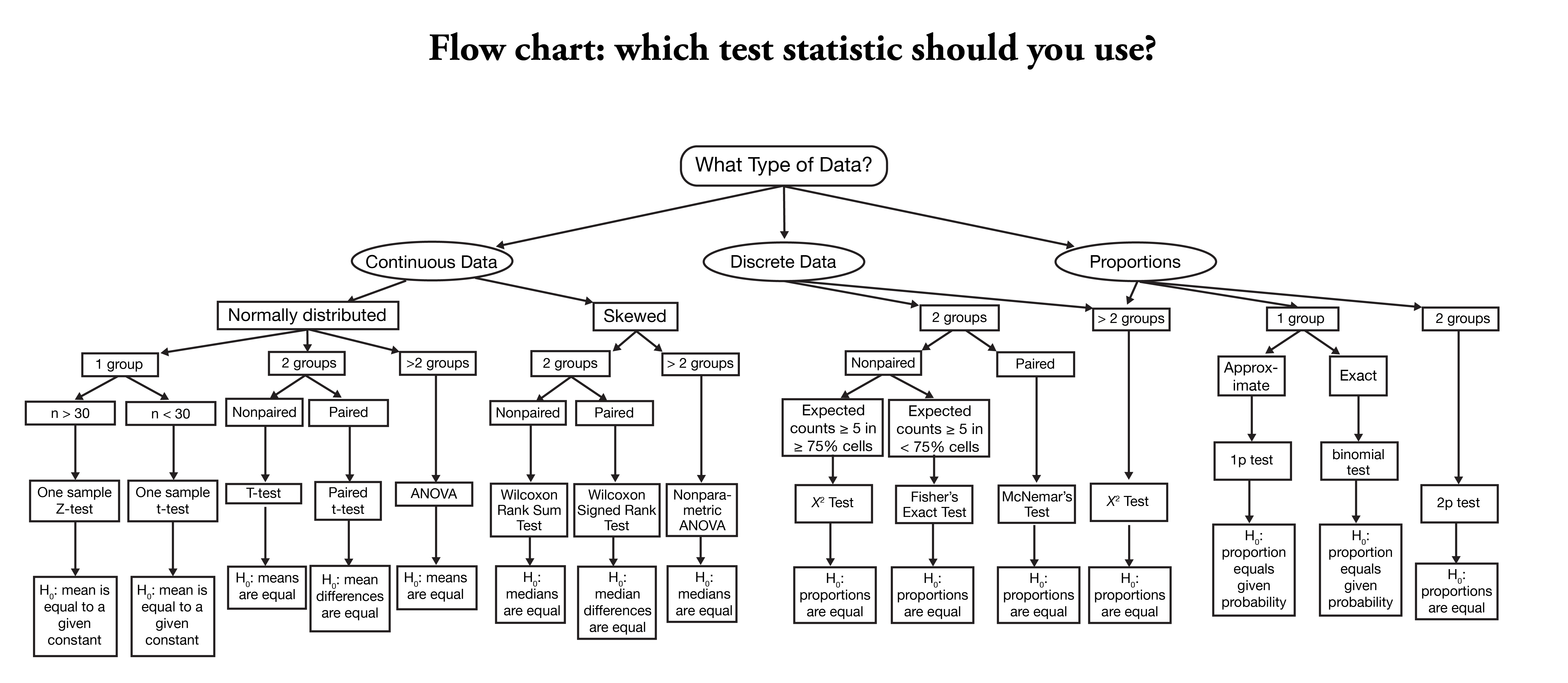
HYPOTHESIS TESTING

Most of the time we are examining two possibilities or two hypothesis, though in some cases we are comparing more than 1 case.  A statistical test lets choose between two competing hypotheses. Similarly confidence intervals reflect the likely range of a population parameter. Scientific investigations start by expressing a hypothesis. Example: Mackowiak et al. hypothesized that the average normal (i.e., for healthy people) body temperature is less than the widely accepted value of 98.6°F. If we denote the population mean of normal body temperature as μ, then we can express this hypothesis as μ < 98.6. From this example:

• We refer to this hypothesis as the null hypothesis and denote it as H0.
• The null hypothesis usually reflects the “status quo” or “nothing of interest”.

In contrast, we refer to our hypothesis (i.e., the hypothesis we are investigating through a scientific study) as the alternative hypothesis and denote it as HA. In simple terms:

• HA : μ < 98.6
• H0 : μ = 98.6

Many of the statistical tests use a time-tested paradigm of statistical inference. In this paradigm, it usually:

• Has one or two data samples.
• Has two competing hypothesis.
  • Each of which could be true.
• One hypothesis, called the null hypothesis, is that nothing happened:
  • The mean was unchanged
  • The treatment had no effect
  • The model did not improve
• The other hypothesis, called the alternative hypothesis, is that something happened:
  • The mean rose
  • The treatment improved the patient’s health
  • The model fit better

Lets say we want to compare something to the default or null expectation

• First, assume that the null hypothesis is true
  • Then, calculate a test statistic. It could be something simple, such as the mean of the sample, or it could be quite complex.
  • Know the statistic’s distribution.Know the distribution of the sample mean (i.e., invoking the Central Limit Theorem)
  • Using the statistic and its distribution to calculate a p-value
    • p-value is the probability of a test statistic value as extreme or more extreme than the one we observed, while assuming that the null hypothesis is true.
    • If the p-value is too small, we have strong evidence against the null hypothesis. This is called rejecting the null hypothesis
    • If the p-value is not small then we have no such evidence. This is called failing to reject the null hypothesis.
  • Common convention regarding p-value interpretation:
    • Reject the null hypothesis when p<0.05
    • Fail to reject the null hypothesis when p>0.05
  • In statistical terminology, the significance level of alpha=0.05 is used to define a border between strong evidence and insufficient evidence against the null hypothesis.
  • Conventionally, a p-value of less than 0.05 indicates that the variables are likely not independent whereas a p-value exceeding 0.05 fails to provide any such evidence.

In other words: The null hypothesis is that the variables are independent. The alternative hypothesis is that the variables are not independent. For alpha = 0.05, if p<0.05 then we reject the null hypothesis, giving strong evidence that the variables are not independent; if p > 0.05, we fail to reject the null hypothesis. You are free to choose your own alpha, of course, in which case your decision to reject or fail to reject might be different.

When testing a hypothesis or a model, the p-value or probability value is the probability for a given statistical model that the default (or null) hypothesis is true, where the p-value of less than 0.05 indicating a 5% change the null hypothesis is wrong, and thus one accepts the alternative hypothesis.

Correlation

Correlation is any statistical association, though in common usage it most often refers to how close two variables are to having a linear relationship with each other.

Correlation is often described as correlation coefficient – which can be calculated in different ways depending on whether one believes the underlying data is a normally distributed or not.  When normally distributed, we calculate the Pearson correlation efficient. When this is not the case, one can calculate the Spearman which avoids the tail wagging the dog.

SENSITIVITY, SPECIFICITY, AND REPRODUCIBILITY (ETC)

Prevalence. Prevalence is the proportion of a population who have a specific characteristic in a given time period. To estimate prevalence, researchers randomly select a sample (smaller group) from the entire population they want to describe. Using random selection methods increases the chances that the characteristics of the sample will be representative of (similar to) the characteristics of the population.

• For a representative sample, prevalence is the number of people in the sample with the characteristic of interest, divided by the total number of people in the sample.
• To ensure a selected sample is representative of an entire population, statistical ‘weights’ may be applied. Weighting the sample mathematically adjusts the sample characteristics to match with the target population.
• Prevalence may be reported as a percentage (5%, or 5 people out of 100), or as the number of cases per 10,000 or 100,000 people. The way prevalence is reported depends on how common the characteristic is in the population.
• There are several ways to measure and report prevalence depending on the timeframe of the estimate.

Incidence. Incidence is a measure of the number of new cases of a characteristic that develop in a population in a specified time period; whereas prevalence is the proportion of a population who have a specific characteristic in a given time period, regardless of when they first developed the characteristic.

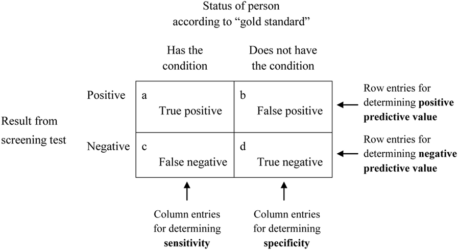
Sensitivity and specificity are statistical measures of the performance of a binary classification test or classification function:

• Sensitivity (true positive rate)
  • measures the proportion of actual positives that are correctly identified as such.
  • Example: the percentage of sick people who are correctly identified as having the condition.

Application to screening study:

• Imagine a study evaluating a new test that screens people for a disease.
• Each person taking the test either has or does not have the disease.
• The test outcome can be positive (classifying the person as having the disease) or negative (classifying the person as not having the disease).
• The test results for each subject may or may not match the subject’s actual status.
  • True positive: Sick people correctly identified as sick
  • False positive: Healthy people incorrectly identified as sick
  • True negative: Healthy people correctly identified as healthy
  • False negative: Sick people incorrectly identified as healthy

Terminology

• Reproducibility – the ability to achieve the same results by repeating the same set of actions independently
• Accuracy—the ability of a test to most closely measure the “true” value of a substance
• Precision—the reproducibility of a test result
• Test sensitivity—the ability of a test to detect a substance especially at relatively low levels
• Test specificity—the test’s ability to correctly detect or measure only the substance of interest and exclude other substance

Below are shown two standards matrix’s for calculating accuracy, precision, etc.  One factor that determines whether to use the upper or lower is based on the concept of prevalence. If we are evaluating a test whereby the number of True Positives and True Negatives are not sampled randomly from the population, we need to know the prevalence of a disease.  An example would be a glioma test where a lab has been tested on 50 Verified True Cases and 50 Verified False Cases. If we calculate PPV or precision from that data, we have not actually considered the prevalence in the population.   Let’s say the test gave 1 false positive for this set of 100 cases – a false positive rate of 1%.  Glioma is actually quite rare only 3 in 1000 will have it.

In the real world, if 1000 get this test with a false positive rate of 1%, we would expect 10 false positives and 3 true positives.  PPV takes this into account, and thus the PPV is actually 23%.

Studying a population (or a prospective study where cases/controls are not defined retrospectively), we can calculate PPV without prevalence because its inherent to measurement of false positives and true positives.  For example TP/(TP+FP)=PPV.

{
  library(ggplot2)
  library('RColorBrewer')
  library(dplyr)
  library(plotly)
  
}

{
  setwd(dir = '~/trgn510/')
  genotypes <- read.csv('kg.genotypes.csv',header = TRUE, sep = ",", 
                           quote = "\"", dec = ".", fill = TRUE, row.names = 1)
  population_details <- read.csv('kg.poplist.csv',header = TRUE, sep = ",", 
                                 quote = "\"", dec = ".", fill = TRUE)
  PopList <- data.frame(population_details[,c(3,2,1)])
}  # Load in Data

{
  genotypes_mini <- as.data.frame(genotypes[c(rep(FALSE,10),TRUE),c(1:500) ])
}
{
  pca_anal <- prcomp(genotypes_mini)
  #st <- data.frame(pca_anal)
  rotation <- data.frame(Sample=row.names(pca_anal$rotation), pca_anal$rotation[,1:6],row.names = NULL)
  people_PCA_diversity<-left_join(PopList,rotation, b, by = "Sample")
}  # End of PCA

plot_ly(people_PCA_diversity, x = ~PC1, y = ~PC2, z = ~PC3, colors="Set1",
        color = ~Population,type="scatter3d",mode="markers")