Historical High Performance Computing

What is high performance computing in the context of bioinformatics?

Biomedical informatics involves big data. One of the biggest drivers lately is genomics and sequencing. Lets go with that example. Aligning a genome is a problem that is easy to break up. Aligning 1 read doesn’t impact aligning another read. If I have 1 billion reads, and a single CPU can align 2500 reads per second it will take 72 hours. If you want the answer quicker you need to split the analysis up and send it off to different computers that ideally all share network storage so that we can keep track of data. This is solved by High-Performance-Computing.

At this point, we should highlight there are three major areas of HPC that bioinformatics sees:

(1) Problems that can be easily broken up – divide and conquer. Analysis of genomes is a great example. Divide and conquer works well when the core calculation doesn’t require knowing what the result is from other calculations. For example, aligning 1 read to a genome, frequently (except for assembly), aligns to the same position in the genome regardless of what everyother read aligns. This is true at least at early steps, and thus we can take a very large file of reads of data and split up the work such that each computer is told to work on a subset of reads. In some programs this can lead to several independent alignment files or BAMs, that must be put together and sorted. Sorting of course would require each read knowing the location of all others – fortunately it is fast enough not to require splitting up across nodes. We will see this by example later.

(2) Problems that require lots of communication at each step & are less easy to break up. Molecular modeling and dynamics is the most relevant example where the positions and velocity of atoms are known, the forces interacting between them are known based on their location, and one wishes to move them all an infinitesimal small step forward based on this info, then recalculate the forces once the atoms have moved. In this scenario, we need to know where all the atoms (x,y, z in cartesian space) are and their current velocity (v), calculate where they will be 1 picosecond later by integrating Force=mass*acceleration, where acceleration is dv/dt. Millions of atoms interacting may take up to 1s across dozens of computers to calculate, but they all need to report back their updated position to calculate the next picosecond. That requires lots of communication at every second since each ps is typically 1 to 500 milliseconds, and this is done often using MPI (Message Passing Interface). Example of titin unfolding visualized in VMD, but run with NAMD. NAMD is the package which does the MPI molecular dynamics.

(3) Problems that be done on GPUs (rarely relevant and development area). Very few applications today use GPUs. These are basically video cards where each one has 1000s of processors but with very little memory. They are largely an area of development and very little to any routine analysis is done on them for applied biomedical informatics at this point.

Lets focus on application #1 – analysis of genomes. Lets just consider the size to help us understand why your laptop may not be sufficient and you need industrial sized computing.

First, how much data is typical for 1 person’s genome?

First lets think about the data size and get perspective. The raw data for sequencing a person genome at 30x is 100 billion bases, where each base has a call and a quality measure of that call. Typically, 100Gb or more. 30x sequencing of a 3 billion base genome produces a lot of data. Lets talk about analysis starting at raw-data level. Typically, we sequence a small fragment of DNA – perhaps a 300 base segment – reading the first 100 bases and last 100 bases. For the germline (or inherited genome) above that is 1 billion reads. The first step is usually aligning those sequences to the reference genome. Remember we aren’t just aligning we are aligning data that will be slightly different. The person we sequencing will have variants, and thus we have to allow mismatches, insertions and deletions. Moreover, there will be error. The reads aren’t perfect but about 99.5% accurate meaning that typically there are 1 to 2 machine errors per read. As a result, its good to sequence multiple times because one typically wants to get to six sigma – or 1 in 1 million accuracy. So if you have 100 or so individuals, and you have 10 terabytes on your hand.

Bioinformatics is big data – but where in the big context?

The simplest unit is Boolean – 0 or 1 and is a bit.
A character is a single byte – “A” is one byte and typically 8 bits
An email contains thousands of bytes
The Nintendo 64 had 4096 bytes of memory
The C64 had 64,000 bytes
The first 5.25″ floppies were 640,000 bytes
The smaller 3.5″ had typically 1-3 Mbytes
An MP3 is 3 to 4 Mbytes.
A microarray often produces 60 Mbytes of data (bioinformatician hour)
A CD-rom stores 600 million bytes;
A DVD is 6 billion bytes or gigabytes (GB)
Flash USB storage can hold 8 to 64 Gbytes
A 30x genome is 100-300 billion bytes for the BAMs and FASTQs(bioinformatician week)
Portable hardrives have about 2 trillion bytes (2 Terabytes or 2TB)
100 individuals ($100K in reagents) requires 30 trillion bytes (30 Terabytes)(bioinformatician year)
Amount of data indexed by Google monthly is 200 Terabytes by approximately 30,000 software engineers
1 NovaSeq 6000 will produce 365 Terabytes per year at full capacity (2 to 3 bioinformatician )
CERN study of “God particle” for Haldron Collider generates 5 Petabytes/yr (1000 Terabytes)
All the internet data 8000 Petabytes

So its not unusual for a lonely bioinformatician or two to be analyzing and managing data sizes (10-200 TB) that are an order or two in magnitude away from what is largely considered the most data rich scientific activity – the search for God particles through the CERN by 1000s of scientiusts, or what we often think of as the interpret (the 0.004% that is being indexed by Google). Hundreds of terabytes is a lot of data.

So what does in terms of processing power, let alone storage to align 1 billion reads in your 30x genome? BWA is the name of a very fast and accurate aligner. It can align 2500 reads per second, and it would take about 75 hours. What if you want it faster? Well we could split it up and have a few computers work on alignment. This frames High Performance Computing (HPC) for bioinformatics. Speaking broadly first, HPC is typically an environment with lots of “computers” or rather “compute nodes” all networked together with lots of bandwidth between them, enough memory to run the calculation, and data storage to put the data.

That much data, we need to think about how long even moving it will take.
How long does it take to transfer 1 person’s whole-genome data?

3G/4G ~ 70 hours
Cable Modem (50 Mbit) ~ 30 hours
USB – 1 to 3 hours with standard USB, though newer USB is Gigabit+.
T3 University to Amazon ~ 1 to 3 hours (some parallel and high-end transfer, but you are saturating tyupical ports).
Pragmatically, its hard to move faster than 400 Mbit to 800 Mbit for a given file across the internet

Key HPC Concepts

More exactly HPC has a few important concepts bioinformatics must know well, and we start by providing a key question driving why that concept matters.

(1) Compute nodes.

Example Question: How many computers and how many cores do they have?

(2) Bandwidth (i/o)

Example Questions: How long does it take to read and write data, particularly if lots of processors or writing and reading on shared storage? How do we get the data into the HPC system?

(3) Memory

Example Question: How much do we need to put into memory – surely, a 3 Gbyte human genome is difficult to put into 2Gb of memory.

(4) Storage.

Example Question: How much storage do we need – where is it and how is it maintained and managed. Where do we put data before and after.

Lets learn about each of these by understanding your personal laptop. In the upper left hand corner of your screen press the apple icon, and select “About this Mac”. We see information about processors, Memory, and Graphics. Lets go deeper by clicking on System Report and look at Hardware Overview.

Your laptop is like a compute node. We can see in the example below this laptop has an Intel Coreil at 2.7Ghz with 1 processors and that processor has 4 cores. Each core can handle a thread. A thread would be for example a script (noting you can always spin off more process within your script using &, and sending to background). We have 16 Gb of memory with 8Mb of L3 Cache and 256 of L2 Cache. These latter two are important, but the key for us is the 16 Gb. The more memory the more things we can open at once – more windows, etc.

We can also click on storage from the “About our Mac” and see how much storage we have and how much is being used. Storage isn’t active – its like having a lot of music on a portal MP3 player – except MP3s take up a little bit space. In this case I have 500 Gb of flash storage. Flash storage is fixed and doesn’t involve a spinning disk – your new iPhone and your iPads are flash, and the original large iPods were spinning disks. Spinning disks usually hold more – they also and always eventually break.

Job Managers (slurm, etc)

The HPC needs a mechanism to distribute jobs across the nodes in a reasonable fashion; this is the task of a program called a scheduler. This is a complicated tasks: the various jobs can have various requirements ( e.g. CPU, memory, diskspace, network transportation, etc. ) as well as differing priorities. And because we want to enable large parallel jobs to run, the scheduler needs to be able to reserve nodes for larger jobs (i.e. if an user submits a job requiring 100 nodes, and only 90 nodes are currently free, the scheduler might need to keep other jobs off the 90 free nodes in order that the 100 node job might eventually run). The scheduler must also account for nodes which are down, or have insufficient resources for a particular job, etc. As such, a resource manager is also needed (which can either be integrated with the scheduler or run as a separate program). The scheduler will also need to interface with an accounting system (which also can be integrated into the scheduler) to handle the charging of allocations for time used on the cluster. There are two major types – Slurm and Torque, and Slurm is becoming more popular. They inessense are shell scripts that contain header information that get to sent to a node, and are run where the directory tree is similar to the head node (where you log in). You then manage the job watching as files appear on a shared disk system. Since files are big, we need to think carefully about management.

As an user, you interact with the scheduler and/or resource manager whenever you submit a job, or query on the status of your jobs or the cluster as a whole, or seek to manage your jobs.

https://carc.usc.edu/user-information/user-guides/high-performance-computing/discovery/slurm-templates

Data Management: Digging deeper

Everything that is glass will probably break, and all disks will fail. Data is expensive to create, and a bioinformaticians job is to often maange data. Losing data can and is a massive problem – it can cost millions, it can cost time, it can get people fired, and with certain types of health data you can be prosecuted. Its a bioinformaticians job to work with IT and scientists to make sure that the risks are known and what the current strategies are. If data isn’t backed up, it is a roll of a dice typically of when that data will be irrecoverably lost. Documentation is key, and processes are key.

Critical data should be backed up in two geographically different locations. Fortunately we live in the era of cloud computing – that is on demand storage managed by IT professionals available in $0.007 increments (store 1 Gbyte for 1 month, and you get charged a fraction of a cent at Amazon). I’ve seen companies get shut down because of water sprinklers triggering a fire. In this sense data management costs significant amount of dollars, and done poorly the expense can be massive.

Lets dive into a High Performance Computing (HPC) environment. In HPC, there is local storage and various networked storage. Network storage is usually not on your computer and is somewhere on the network. That means if its say at a location with just a little bandwidth, it’ll be slow to load on your computer. There are typically hundreds to thousands of CPUs reading from this storage, and they very easily can use up bandwidth. Thus there are a different types of storage and we do need to know more about them in bioinformatics. Now its important to know that these are rarely a single drive, but rather many many drives where data from your project is written across them somewhat redundantly. RAID storage is this – your data is striped across a bunch of drives and provides two advantages. First it helps spread out the bandwidth so that you can get simultaneously read across lots of drives. Second, if a drive files there is typically enough redundancy that you are fine and your data isn’t lost.

Critical network storage servers types

Each HPC environment has their own setup, but there is convention – and frequently common themes about which data storage is meant for calculation and temporary storage and which data storage is for long-term storage, etc. On any computer you can always see what’s mounted by ‘df -h’. The list is long, and only a few are really critical – scratch, long-term storage, and your home directory. These are often served to your computer on different servers, and then mounted made available by a simple ‘cd /yourServer‘. Alias’s and links can sometimes mask when you switch storage – so one must be careful so as to not run out of space. This frequently occurs by newbies or new users storing all their data in their home directory. Often this space is small -purposely so – to keep you from hoarding data where you shouldn’t.

Stratch or Staging Storage. This is typically large continuous data. Its often optimized to handle lots of computers reading and writing tons of data simultaneously. Its also met to be temporary storage, so there is less redundancy. Often when we are doing an analysis we will read and write to a scratch storage.

df -h | grep staging

beegfs_nodev 328T 312T 16T 96% /staging

Long-term storage. Staging is another continuous block of data storage. It is optimized for you to upload your datafiles once, and your data is safe there for short-periods of times.

ln -s/auto/dtg-scratch-01/dwc3/davidwcr/ ~/storage

#To get to our storage, thus cd ~/storage

Home storage. This is the storage that holds your home directory and some of the files and programs you use. Its usually not that big, and you shouldn’t really upload large datasets.

davidwcr@hpc-login3:~ df -h | grep rcf-40

almaak-05:/export/samfs-rcf/rcf-40 5.5T 2.1T 3.5T 37% /auto/rcf-40

Other types of data storage

Glacial storage. This is a long-term back-up option where you don’t need data but very rarely, and its effectively written to a storage type that can take hours to retrieve, but the cost of storage is very cheap

Cloud storage. This is storage typically at a commercial vendor such as Google or Amazon – but under the hood the storage is typically not that different from some of the other storage types above, other than we need a networked connection to Google.

Local storage. Each node or computer usually has a small amount of storage built in – typically from a hard-drive and sometimes you want to use it for data that needs to move back and forth a lot between disk and memory.

Tape storage. This is usually for long-term backup, where it can take hours to weeks to get data from tape. These literally are tapes, and sometimes its robots that go and get the right tape and sometimes its humans.

There are often many many other types of storage. One way to see all the storage available is to login and type “df -h”.

Data needs to be organized. Primary data should be in an logical order and hierarchal

SETTING UP A SERVER VIA GOOGLE CLOUD

This is an optional path. You will need a Google Cloud account to proceed, and you should note that there is a cost associated with serving via your own server. I provide this as a path, but note that folks will be able to use a default cloud account without cost.

Create Virtual Machine (VM)

Click Compute Engine, Instance templates.

Press create to create an instance.

Change the Boot disk to Centos 7, click Allow HTTP traffic and Allow HTTPS traffic, then hit create. We don’t know the memory your app will take yet, but you can monitor and change appropriately.

Click ssh and it will open up a web-based console automatically setting up keys.

You are given an account, and the ability to install root software. You will also get your IP. This is important. In this case the IP is 35.192.117.51.

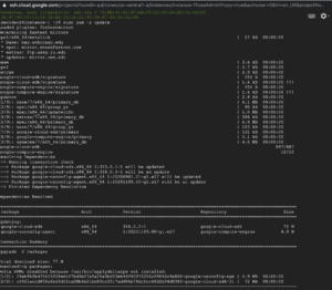
We need to install some default software, and update the system.

Setup the linux server security and updates

sudo yum -y update 
sudo yum -y install epel-release wget git mod_ssl nginx zlib-devel libxml2-dev gcc libcurl4-openssl-dev libssl-dev mod_ssl openssl xml2 curl openssl-dev libcurl-devel

This will take 5 to 10 minutes….

Allow SSH (optional)

We won’t be able to ssh in without our Google console, so lets enable password authentication.

Now we need to enable logins via ssh, please sudo vi /etc/ssh/sshd_config

Editing /etc/ssh/sshd_config

Change PasswordAuthentication no to PasswordAuthentication yes

write and quit, esc :wq

Restart the sshd

sudo service sshd restart

By default, shiny uses port 3838. If we want this open to the world, we need to open the firewall port

sudo firewall-cmd --permanent --zone=public --add-port=3838/tcp
sudo firewall-cmd --permanent --zone=public --add-port=4151/tcp
sudo firewall-cmd --permanent --zone=public --add-service=http
sudo firewall-cmd --permanent --zone=public --add-service=https
sudo firewall-cmd --reload

LEARNING HPC THROUGH ALIGNMENT OF EXOME.

Lets conduct a basic pipeline analysis. In this case we are going to call the genetic variants from 1 person within their coding region (exome). We will need to go from raw data to variants by aligning the raw data to the reference genome. We have 3 major file types FASTQs (raw data), BAMs (Aligned Reads), VCFs (Called variants). In this process we are lessed concerned with the details of the biology then the steps in doing an analysis.

We will need to:

Setup our server for a pipeline
Get our raw sequencing data via a dataserver.
Install our programs or insure that they are available (samtools & BWA)
Download & Setup up our common resources – (download and index B37 of the human genome)
Align reads to create a BAM from the FASTQs using BWA
Call variants to create a VCF from the BAMs. The VCF is what we are looking for.
Annotate VCFs so that we know what the variants do. (Not available yet)
Put all of this in a single pipelined script – This is assignment (due date April 16th).

Step 0. Login to server and setup

You will need to use your original server – you can use Google console or login via your IP

ssh yourname@12.12.12.32

Step 1. Setup our Server for a Pipeline

First lets login our server by ssh’ing into our server (change trgn510 to your username), and lets look at our disks using df -hk

df -h

The out put should be something like

Filesystem      Size  Used Avail Use% Mounted on
/dev/sda1      1000G   32G  969G   4% /
devtmpfs         13G     0   13G   0% /dev
tmpfs            13G     0   13G   0% /dev/shm
tmpfs            13G  385M   13G   3% /run
tmpfs            13G     0   13G   0% /sys/fs/cgroup
tmpfs           2.6G     0  2.6G   0% /run/user/1001

Step 2. Get our raw sequencing data via a dataserver

(Retrieving The Raw FASTQs for our person)

Downloading Exome Data From NA12878

First lets make sure we are on the right server or node. Only hpc-transfer is optimized for data transfer, and it sees the entire internet. We are only going to look at an exome – basically where the coding regions have been enriched and we largely are only sequencing 1% of the genome. For learning and many applications this is fine.

Lets organize our data – note that you can replace $USER with your username or you can use that variable call itself.

mkdir -p ~/fastqs/na12878/exome/giab
cd ~/fastqs/na12878/exome/giab/

We would like to download several files and they’ll each take a while. Lets put this in a bash script. In VIM, create a script called download_na12878.sh. You can paste the following lines in, where it will consecutively download them from Genome in a Bottle. If you do copy and paste this, appreciate that normally you would have to create this yourself – and its never very elegant (lots of copy of pasting). I’m using curl this time because variety is good. Create the script download_na12878.sh

mkdir ~/scripts

vim ~/scripts/download_na12878.sh #(create in vim)

Paste below into your script directory.

~/scripts/download_na12878.sh

#!/usr/bin/bash
cd ~/fastqs/na12878/exome/giab/
curl -O ftp://ftp-trace.ncbi.nih.gov/giab/ftp/data/NA12878/Garvan_NA12878_HG001_HiSeq_Exome/NIST7035_TAAGGCGA_L001_R1_001.fastq.gz
curl -O ftp://ftp-trace.ncbi.nih.gov/giab/ftp/data/NA12878/Garvan_NA12878_HG001_HiSeq_Exome/NIST7035_TAAGGCGA_L001_R2_001.fastq.gz
curl -O ftp://ftp-trace.ncbi.nih.gov/giab/ftp/data/NA12878/Garvan_NA12878_HG001_HiSeq_Exome/NIST7035_TAAGGCGA_L002_R1_001.fastq.gz
curl -O ftp://ftp-trace.ncbi.nih.gov/giab/ftp/data/NA12878/Garvan_NA12878_HG001_HiSeq_Exome/NIST7035_TAAGGCGA_L002_R2_001.fastq.gz
curl -O ftp://ftp-trace.ncbi.nih.gov/giab/ftp/data/NA12878/Garvan_NA12878_HG001_HiSeq_Exome/NIST7086_CGTACTAG_L001_R1_001.fastq.gz
curl -O ftp://ftp-trace.ncbi.nih.gov/giab/ftp/data/NA12878/Garvan_NA12878_HG001_HiSeq_Exome/NIST7086_CGTACTAG_L001_R2_001.fastq.gz
curl -O ftp://ftp-trace.ncbi.nih.gov/giab/ftp/data/NA12878/Garvan_NA12878_HG001_HiSeq_Exome/NIST7086_CGTACTAG_L002_R1_001.fastq.gz
curl -O ftp://ftp-trace.ncbi.nih.gov/giab/ftp/data/NA12878/Garvan_NA12878_HG001_HiSeq_Exome/NIST7086_CGTACTAG_L002_R2_001.fastq.gz

We can then chmod 755 download_na12878.sh.

chmod 755 ~/scripts/download_na12878.sh

Run the script with output going to screen:

~/scripts/download_na12878.sh >& ~/scripts/download_na12878.out &

The “&” at the end sends it to background. The >&redirects the output from the screen to `~/scripts/download_na12878.out`

We can check the progress using tail -f

tail -f ~/scripts/download_na12878.out

Side note 1. As we wait, its important to be aware how big a file is and how small. Its also important to know Mb/s is Megabit and MB/s is Mergabyte. Roughly, but not accurately 1 MB/s=8 Mbit/s or 8 megabit per second. A typical home line is 50 Mbit or 8 Mbyte/s. A 100 Mbit cap is frequent due to their frequent use in routers and is typically found where you see 25 MB/s (megabytes/s). A Gigabit connection gets you 100-150 MBytes/s and that’s frequently hard to get because your data frequently leaves harddrive at less than speed. To get that you usually have to use special protocols that use multiple connections, and use different protocols (UDP vs. TDP).

Sidebar – Since you may be waiting lets talk some about this person, NA12878, references within clinical labs are samples that can be used to estimate reproducibility and accuracy for a laboratory tests performance. This data is at Genome in a Bottle and is their effort at getting to a better reference. This is not the reference genome that is used to align again! Don’t get confused – that is another person or rather 8 different people, but mostly someone from Rochester, NY. Rather we want to know how good we are measuring differences from the reference genome, and we need a “gold star” reference – once person to be that individual that is sequenced again and again to check reproducibility. Yes, that term reference gets used a lot, so try to not get confused. In this case, references samples (unlike the reference genome) are created by groups such as NIST – and we are downloading from them one person who has become essentially the closest to a consensus reference sample, NA12878 out there because she’s been sequenced so much and by so many people. This person was selected from the well established CEPH cohort in 1984 . The CEPH cohort (Centre d’Etude du Polymorphisme Humain) was established years ago, and cells from them have been immortalized. The goal of CEPH was to initiate and lead an international collaboration in order to establish the first genetic map of the human genome. To achieve this, a collection of DNAs from 40 large Utah Mormon families were enrolled. For some CEPH individuals with larger families it is possible using just a little additional information, and this is of course one challenge with her use. However, its not that simple. To be a reference, ideally you have consented for this. NA12878 – a female consented for research use only and not for commercial use. This makes her use for validating assays as the gold standard such as for in vitro diagnostics sub-optimal. We can see she had 6 boys and 6 girls. How unique do you think she is – 6 boys and 6 girls from Utah? Is it possible to re-identify her if you had birth records?

There are other more broadly consented individuals who have consented to releasing their data free and clear, for profit or not, for any one and any country and for any purpose. Still those individuals have not been sequenced as many times by as many groups and by as many technologies. There may be only one other person who has been sequenced as fully – using newer technology and older Sanger based – and they may be the last and only – Craig Venter who led 1 of 3 groups to sequence and build the first map competing with the French and NIH. His brash approaches and questions about data ownership from the original Celera do pose historical questions. Till then NA12878 is the best and closest to a reference sample we have. Craig Venter, Jim Watson, and a Yriban family (NA19240) are others that have been sequenced by many technologies. Jim Watson though retracted parts of the genome – namely the Alzheimer’s locus to protect in part family members from any bias. Still, researchers were able to show that could estimate his ApoE-e4 status, and so a few more chunks were redacted.

You should have your raw data by now. You could actually do a check, by reducing some very large files to a signature, called an MD5 hash. This is done by running md5sum on the sample and a short hash will be created. Please do this as I do. What if there was a glitch – or an incomplete transfer? How do we know we have the data? The primary way is through calculation of md5sum and running that program on the entire dataset.
md5sum NIST7035_TAAGGCGA_L001_R1_001.fastq.gz
630c611d62d995c5aeb60211add2f26e NIST7035_TAAGGCGA_L001_R1_001.fastq.gz

The result “63…6e” for NIST7035_TAAGGCGA_L001_R1_001.fastq.gz should be the same – and indeed we can check that NIST got the same MD5SUM by looking in their repository at their MD5s. This allows a path to ensure that we actually transferred these files and they are identical. In practice, people also simply use filesize as a match. However – this doesn’t always work – though using file sizes does save time. Different disk systems may give different filesizes for the identical files due to hour they store them adding overhead. Both filesizes and MD5’s are used in the field – where filesize is used with caution when its safe to assume the filesizes and disks are the same.

You can see my filesizes below:
1869888 -rw-rw-r-- 1 davidwcr lc_dwc3 1914722761 Oct 19 13:42 NIST7035_TAAGGCGA_L001_R1_001.fastq.gz
1909120 -rw-rw-r-- 1 davidwcr lc_dwc3 1954935121 Oct 19 13:42 NIST7035_TAAGGCGA_L001_R2_001.fastq.gz
1916544 -rw-rw-r-- 1 davidwcr lc_dwc3 1962477139 Oct 19 13:44 NIST7035_TAAGGCGA_L002_R1_001.fastq.gz
1954304 -rw-rw-r-- 1 davidwcr lc_dwc3 2001172486 Oct 19 13:44 NIST7035_TAAGGCGA_L002_R2_001.fastq.gz
1990208 -rw-rw-r-- 1 davidwcr lc_dwc3 2037956271 Oct 19 13:45 NIST7086_CGTACTAG_L001_R1_001.fastq.gz
2032640 -rw-rw-r-- 1 davidwcr lc_dwc3 2081364133 Oct 19 13:46 NIST7086_CGTACTAG_L001_R2_001.fastq.gz
2034688 -rw-rw-r-- 1 davidwcr lc_dwc3 2083510543 Oct 19 13:47 NIST7086_CGTACTAG_L002_R1_001.fastq.gz
2075712 -rw-rw-r-- 1 davidwcr lc_dwc3 2125471805 Oct 19 13:48 NIST7086_CGTACTAG_L002_R2_001.fastq.gz
Or in human readable by ls -lh, we see the file sizes are indeed smaller with an exome. For those who are used to the wet-lab and how Illumina flow-cells work, we also see this person was sequenced across two different lanes of a flowcell, and that they used molecular barcodes. We also see the R1 and R2 reads – these are paired reads. Lets examine the first 5 rows of two of these files – one from the forward and one from reverse.
gunzip -cd NIST7035_TAAGGCGA_L001_R1_001.fastq.gz | head
 @HWI-D00119:50:H7AP8ADXX:1:1101:1213:2058 1:N:0:TAAGGCGA
 ACTCCAGCCTGGGCAACAGAGCAAGGCTCGGTCTCCCAAAAAAAAAAAAAAAAAAAAAAAATTGGAACTCATTTAAAAACACTTATGAAGAGTTCATTTCT
 +
 @@@D?BD?A>CBDCED;EFGF;@B3?::8))0)8?B>B@FGCFEEBC######################################################
 @HWI-D00119:50:H7AP8ADXX:1:1101:1242:2178 1:N:0:TAAGGCGA
 ACATAGTGGTCTGTCTTCTGTTTATTACAGTACCTGTAATAATTCTTGATGCTGTCCAGACTTGGAATATTGAATGCATCTAATTTAAAAAAAAAAAAAAA
 +
 @@@DDBAAB=AACEEEFEEAHFEEECHAH>CH4A<+:CF<FFE<<DF@BFB9?4?<*?9D;DCFCEEFIII<=FFF4=FDEECDFIFFEECBCBBBBBB>5
 gunzip -cd NIST7035_TAAGGCGA_L001_R2_001.fastq.gz | head
 @HWI-D00119:50:H7AP8ADXX:1:1101:1213:2058 2:N:0:TAAGGCGA
 NNNNNAGGGNGGACNCNNTGANAGGAAGAAATGACNTCTTCCTAAGTGTTTTTAAATTACTTCCATGTNNNNNNNNNNNNNNNNNNNNNNNNNNNNNNNNN
 +
 #####-28@#4==@#2##32=#2:9==?<????=?#07=??=??>?>?>??<;?????>?@@=>?####################################
 @HWI-D00119:50:H7AP8ADXX:1:1101:1242:2178 2:N:0:TAAGGCGA
 CCCTTAGTCATTAAAGAAAATGTTTGTATTCTTTTTTTTAATGTGGATGAATGTTTGCTTTTTTTTTTTTTTTAAATTAGATGCATTCAATATTCCAAGTC
 +
 ???DDFDFDHHHDIJJJJGIGIIIJIIGIIEIIIJJJJJHHIIIHIDGIICGHJGJHBGHGIIHFDDDDDDDB?>3:@:+:44((4@:AA:3>C:@CD::3
You can see that consistent with fastq files, there are 4 lines per read in each file, and the reads are ordered such that they match in the R1 and R2 (forward and reverse reads. Line 1 is the name the read “@HWI…GGCGA” is the name of the read, following illumina convention that tells the exact location of that spot leading to our sequence. We can see the sequence read from 5->3, noting that ATCG and N are possible, where N is an unknown. We can see the direction by a + in row 3. In row 4 we see a quality score that is ascii encoded. ASCII encoding is a way to encode the PHRED scaled quality where the error is implied by 10^-PHRED score divided by 10 – or more simply PHRED of 10 is 90% probability of correct, 20 is 99%, 30 is 99.9% and so forth. You can learn to decode from the wikipedia page.You can also use an ASCII table yourself and just subtract 33. We see that the “#” is not so good since 35-33 is 2, and 10^.2 is basically 25% a 1 in 4 chance.

Step 3. Install (compile) our programs or insure that they are available (samtools & BWA)

BWA install we are generally following: https://github.com/lh3/bwa

Compiling programs for local usage.

Ideally programs are compiled and working for us within our pipeline. Sometimes they may not be, and we have to build them ourselves from the raw code. Compiled code, unlike scripts is turned into machine language and every architecture of machine can be different. This means that the conversion to machine code, requires that we compile whenever we are on a different operating system/cpu. For example MacOS is different the Centos/Linux.

BWA

Lets compile a local copy of BWA.

mkdir -p ~/bin/bwa_build
cd ~/bin/bwa_build
git clone https://github.com/lh3/bwa.git
cd bwa; make

To get this to work you’ll need to add git… sudo install git

Example output at the end:

gcc -c -g -Wall -Wno-unused-function -O2 -DHAVE_PTHREAD -DUSE_MALLOC_WRAPPERS utils.c -o utils.o
gcc -c -g -Wall -Wno-unused-function -O2 -DHAVE_PTHREAD -DUSE_MALLOC_WRAPPERS kthread.c -o kthread.o
gcc -c -g -Wall -Wno-unused-function -O2 -DHAVE_PTHREAD -DUSE_MALLOC_WRAPPERS kstring.c -o kstring.o
gcc -c -g -Wall -Wno-unused-function -O2 -DHAVE_PTHREAD -DUSE_MALLOC_WRAPPERS ksw.c -o ksw.o
gcc -c -g -Wall -Wno-unused-function -O2 -DHAVE_PTHREAD -DUSE_MALLOC_WRAPPERS bwt.c -o bwt.o
gcc -c -g -Wall -Wno-unused-function -O2 -DHAVE_PTHREAD -DUSE_MALLOC_WRAPPERS bntseq.c -o bntseq.o
gcc -c -g -Wall -Wno-unused-function -O2 -DHAVE_PTHREAD -DUSE_MALLOC_WRAPPERS bwa.c -o bwa.o
gcc -c -g -Wall -Wno-unused-function -O2 -DHAVE_PTHREAD -DUSE_MALLOC_WRAPPERS bwamem.c -o bwamem.o

We see that it finishes. We need to see if it works, typing ls we see a program named bwa.

~/bin/bwa_build/bwa/bwa

The output should be something like

Program: bwa (alignment via Burrows-Wheeler transformation)
Version: 0.7.17-r1188
Contact: Heng Li <lh3@sanger.ac.uk>
Usage: bwa <command> [options]
Command: index index sequences in the FASTA format
 mem BWA-MEM algorithm
 fastmap identify super-maximal exact matches
 pemerge merge overlapping paired ends (EXPERIMENTAL)
 aln gapped/ungapped alignment
 samse generate alignment (single ended)
 sampe generate alignment (paired ended)
 bwasw BWA-SW for long queries
shm manage indices in shared memory
 fa2pac convert FASTA to PAC format
 pac2bwt generate BWT from PAC
 pac2bwtgen alternative algorithm for generating BWT
 bwtupdate update .bwt to the new format
 bwt2sa generate SA from BWT and Occ
Note: To use BWA, you need to first index the genome with `bwa index'.
 There are three alignment algorithms in BWA: `mem', `bwasw', and
 `aln/samse/sampe'. If you are not sure which to use, try `bwa mem'
 first. Please `man ./bwa.1' for the manual.

now that it works, lets put a simbolic link in our bin path, so that we don’t need to type the full path each time.

ln -s ~/bin/bwa_build/bwa/bwa ~/bin/bwa

samtools

Samtools install we are following these directions: http://www.htslib.org/download/

samtools is a program that we will use for calling variants and looking at BAMs. We follow the instructions for INSTALL.

mkdir ~/bin/samtools_build # make the directory
cd ~/bin/samtools_build # cd into it
wget https://github.com/samtools/samtools/releases/download/1.7/samtools-1.7.tar.bz2 #download the data
bunzip2 samtools-1.7.tar.bz2 #Unzip it
tar -xvf samtools-1.7.tar #Untar it
cd samtools-1.7 #CD in the directory
./configure #run configure script
make DESTDIR=~/bin/samtools_build/samtools-1.7 # make the compiled program in a local directory

We seem to have compiled ok, ,so we check samtools within the working directory

./samtools

which produces the desired output. Again lets setup a symbolic link in our bin.

ln -s ~/bin/samtools_build/samtools-1.7/samtools ~/bin/

Checking samtools by typing samtools shows it works.

Step 4. Download & Setup up our common resources

First, downloading the reference human genome. The current build of the genome is 38. However, in large part most data still is in build 37 which we will use for now. We will use the version that was used for 1000 Genomes. You’ll notice the gz has an index that is available for programs to reach in and pull information without uncompressing the whole thing. Thus there is the large file and the smaller index, ending in .fai.

mkdir -p ~/resources/b37 
cd ~/resources/b37 
wget ftp://ftp.ncbi.nlm.nih.gov/1000genomes/ftp/technical/reference/human_g1k_v37.fasta.fai
wget ftp://ftp.ncbi.nlm.nih.gov/1000genomes/ftp/technical/reference/human_g1k_v37.fasta.gz

Second, we must build an index for speeding up lookup. An index is typically like the index at the back of a book. A place to go to look up using keywords where in our larger book things are. Lets put this in a script called build_bwa_index.sh

Background Info. You might think that there would be 23 different fasta records – one for each chromosome in this build. There is actually quite a bit more and we can grep out the headers.
cd ~/resources/b37
gzip -cd human_g1k_v37.fasta.gz | grep ">"
>1 dna:chromosome chromosome:GRCh37:1:1:249250621:1
etcWe see unmapped decoys, mitocondrial genome, viral sequences, and others. A human genome contains quite a bit – and we have some wholes where we don’t know where some things fit. These are all represented and different groups add different sequences to help to improve alignment. For example, cervical cancer almost always has HPV infected cells, and thus one would include HPV in the genome for aligning to those specimans. End of the day, even a build has different versions and they are context dependent.

BWA works by first getting a series of best possible matches by taking a quick perfect search of a subset of the sequence, and then doing a more thorough alignment to see exactly how the sequence align. It requires us to build an index or a lookup table for these subsets (or kmers).

At USC, you should know the established most exhaustive way to align a sequence to another is the Smith-Waterman algorithm. I encourage you to understand it conceptually, knowing that it actually isn’t used by BWA which takes a more pragmatic and faster approach of seed and extend from candidates – that is less thorough but actually finishes an exome analysis in a couple days. We’ve estimated full and complete Smith-Waterman of NGS for a genome would be many orders of magnitude longer. In terms of bioinformatics and development of algorithms, Smith-Waterman is arguably the most famous algorithm developed by Mike Waterman when he was at Los Alamos in 1981. Today, Waterman is Chair in USC computational Biology and Bioinformatics department, and this department is largely focused on finding and developing novel computational algorithms, where we are much more applied and must use tools that take pragmatic short-cuts based on heuristic knowledge of what works relatively quickly. Still at the foundation of genomics is alignment – and that algorithm is still the best theory.

To index, we really only need to do this once.

mkdir ~/scripts
cd ~/scripts
vim ~/scripts/build_bwa_index.sh

build_bwa_index.sh

#!/bin/bash
DATADIR="~/resources/b37"
mkdir -p ${DATADIR}
######################################### #  #Running Analysis #########################################
echo Running Analysis
echo Path is `pwd`
cd ${DATADIR}
bwa index ${DATADIR}/human_g1k_v37.fasta.gz

We need to remember to change permissions

chmod 755 ~/scripts/build_bwa_index.sh

We then run it in the background

nohup ~/scripts/build_bwa_index.sh >& ~/scripts/build_bwa_index.out &

Where the & instructs to send the previous command to background and the nohup allows you to logout without killing the job. Now you can logout and come back when indexing.

STEP 5. Alignment From FASTQs to BAMs

Alignment takes multiple steps, and BWA with mem option is a very popular aligner. One question is threading, and sometimes its easiest to spawn off threads on your own by sending to background by ending a line with an amperstamp (&). In the case of multiple fastq we align them in pairs creating a temporary file. This will be put into a script that for now will be a hard coded pbs or slurm script. We add this info.

mkdir ~/scripts
cd ~/scripts
vim ~/ scripts/bwa_align.sh

To align we create an alignment script

bwa_align.sh

#!/bin/bash
# CREATE 4 BAMS (alignment files)
mkdir -p ~/bams/na12878/
cd ~/bams/na12878 # Alignmnet consists of 4 scripts - and we need to align 4 fastqs. Each can be done seperately, and then merged together. 
bwa mem ~/resources/b37/human_g1k_v37.fasta.gz "<zcat ~/fastqs/na12878/exome/giab/NIST7035_TAAGGCGA_L001_R1_001.fastq.gz" "<zcat ~/fastqs/na12878/exome/giab/NIST7035_TAAGGCGA_L001_R2_001.fastq.gz" >>~/bams/na12878/NA12878.NIST7035_TAAGGCGA_L001.sam 2>>error.align1
bwa mem ~/resources/b37/human_g1k_v37.fasta.gz "<zcat ~/fastqs/na12878/exome/giab/NIST7035_TAAGGCGA_L002_R1_001.fastq.gz" "<zcat ~/fastqs/na12878/exome/giab/NIST7035_TAAGGCGA_L002_R2_001.fastq.gz" >>~/bams/na12878/NA12878.NIST7035_TAAGGCGA_L002.sam 2>>error.align2
bwa mem ~/resources/b37/human_g1k_v37.fasta.gz "<zcat ~/fastqs/na12878/exome/giab/NIST7086_CGTACTAG_L001_R1_001.fastq.gz" "<zcat ~/fastqs/na12878/exome/giab/NIST7086_CGTACTAG_L001_R2_002.fastq.gz" >>~/bams/na12878/NA12878.NIST7086_CGTACTAG_L001.sam 2>>error.align3
bwa mem ~/resources/b37/human_g1k_v37.fasta.gz "<zcat ~/fastqs/na12878/exome/giab/NIST7086_CGTACTAG_L002_R1_001.fastq.gz" "<zcat ~/fastqs/na12878/exome/giab/NIST7086_CGTACTAG_L002_R2_001.fastq.gz" >>~/bams/na12878/NA12878.NIST7086_CGTACTAG_L002.sam 2>>error.align4
samtools fixmate -O bam NA12878.NIST7035_TAAGGCGA_L001.sam NA12878.NIST7035_TAAGGCGA_L001.bam >& fix.thread1.log
samtools fixmate -O bam NA12878.NIST7035_TAAGGCGA_L002.sam NA12878.NIST7035_TAAGGCGA_L002.bam >& fix.thread2.log
samtools fixmate -O bam NA12878.NIST7086_CGTACTAG_L001.sam NA12878.NIST7086_CGTACTAG_L001.bam >& fix.thread3.log
samtools fixmate -O bam NA12878.NIST7086_CGTACTAG_L002.sam NA12878.NIST7086_CGTACTAG_L002.bam >& fix.thread4.log
samtools sort NA12878.NIST7035_TAAGGCGA_L001.bam >> NA12878.NIST7035_TAAGGCGA_L001.sort.bam 2>> sort.thread1.log
samtools sort NA12878.NIST7035_TAAGGCGA_L002.bam >> NA12878.NIST7035_TAAGGCGA_L002.sort.bam 2>> sort.htread2.log
samtools sort NA12878.NIST7086_CGTACTAG_L001.bam >> NA12878.NIST7086_CGTACTAG_L001.sort.bam 2>> sort.htread3.log
samtools sort NA12878.NIST7086_CGTACTAG_L002.bam >> NA12878.NIST7086_CGTACTAG_L002.sort.bam 2>> sort.htread4.log
samtools index NA12878.NIST7035_TAAGGCGA_L001.sort.bam >& index.thread1.log
samtools index NA12878.NIST7035_TAAGGCGA_L002.sort.bam >& index.thread2.log
samtools index NA12878.NIST7086_CGTACTAG_L001.sort.bam >& index.thread3.log
samtools index NA12878.NIST7086_CGTACTAG_L002.sort.bam >& index.thread4.log 
# Lets wait till everything is done then merge bams wait samtools merge NA12878.merge.bam NA12878.NIST7035_TAAGGCGA_L001.sort.bam NA12878.NIST7035_TAAGGCGA_L002.sort.bam NA12878.NIST7086_CGTACTAG_L001.sort.bam NA12878.NIST7086_CGTACTAG_L002.sort.bam >& merge.log # the >& sends output and error to log, whereas > only sends output samtools index NA12878.merge.bam >& index.log 
# Lets delete old unneeded intermediate files 
rm *.sort.bam *.sam NA12878.NIST7035_TAAGGCGA_L001.bam NA12878.NIST7035_TAAGGCGA_L002.bam NA12878.NIST7086_CGTACTAG_L001.bam NA12878.NIST7086_CGTACTAG_L002.bam

We run the files via start the script:

mkdir -p ~/bams/na12878/ 
cd ~/bams/na12878 
~/scripts/bwa_align.sh  >&~/scripts/bwa_align.out

If you run it this way (~/scripts/bwa_align.sh >&~/scripts/bwa_align.out) it will hang waiting for the entire script to finish which is several hours. You may want to run it having it go to background so that you can log off by adding the & symbol at the end. For example:

~/scripts/bwa_align.sh  >&~/scripts/bwa_align.out &

The result is are a key pair – NA12878.merge.bam and NA12878.merge.bam.bai

STEP 6. From BAMs to VCFs

This time, I ask you do by following mostly their instructions.

There are many variant callers. A variant caller identifies genetic variants specific to an individual by looking at the alignments in the BAM, GATK. GATK is a java-based program and its slightly different – typically not requiring compiling and in theory should work on all computers. Another is samtools. Another in FreeBayes. We are going to use FreeBayes.

https://github.com/ekg/freebayes

This time I’d like you to install the software. We are going to move from being spoonfed to independence. However,, please make your builds in the following directory to insure we have space:

mkdir -p ~/builds
cd ~/builds

Once you create your build, you can ‘mv’ or ‘ln -s’ to your bin, or alternatively just add the directory to your path. For example: ln -s to ~/bin/, e.g. `ln -s ~/builds/freebayes/bin/freebayes ~/bin/.

You want to call variants using the part on the web page “Call variants assuming a diploid sample:” and this analysis should be done in

~/vcfs/na12878

using a script run in ~/scripts for called run_freebayes.sh

You’ll need to know where your BAM is (na12878.merged.bam), and you’ll need to have a reference.

~/resources/b37/human_g1k_v37.fasta
freebayes -f ~/resources/b37/human_g1k_v37.fasta ~/bams/na12878/NA12878.merge.bam > NA12878.freebayes.vcf

The output file should be called ~/vcfs/na12878/NA12878.freebayes.vcf. and the input should be your file ~/bams/na12878/NA12878.merge.bam

If it doesn’t work – make sure that the prior step was successful. One clue is in your log file.. The other is that you will have a very large BAM file.

To kick this off then – and it will take a few hours we have a few choices.

First type ~/scripts/run_freebayes.sh You will notice it will hang waiting for it to finish. You can press control “z”, then type bg to send to background, and then disown. At that point you could log off and it would keep going.
~/scripts/run_freebayes.sh >& ~/scripts/run_freebayes.log &. The & will send it background, and again you can disown it by typing disown to insure it keeps running when you log off.
You can use nohupfollowed by the & sign. e.g. `nohup ~/scripts/run_freebayes.sh >& ~/scripts/run_freebayes.log &

All three of these will start the program on the server.

STEP 7. Annotate VCFs

Lets figure out what these variants cause. We will use SNPEFF to turn a genomic change into a predicted functional change. The directions for install are here and please use ~/builds for getting your program running, e.g.

mkdir -p ~/builds 
cd ~/builds

Follow “Installing Snpeff” from http://snpeff.sourceforge.net/SnpEff_manual.html#run

This program is a java based program. Java is pre-installed and you don’t run the binary, but rather have java do this. Java programs should coneivably work on every platform with the same “jar” file. The instructions say to run as below within a script called

java -Xmx4g -jar snpEff.jar GRCh37.75 examples/test.chr22.vcf > test.chr22.ann.vcf

This essentially sets a max memory of 4gigs. For annotation, lets use Genome Build 37.75. I’m going to write out the full command as we would need it.

java -Xmx16g -jar ~/builds/snpEff/snpEff.jar GRCh37.75 ~/vcfs/na12878/NA12878.freebayes.vcf >~/vcfs/na12878/NA12878.freebayes.snpeff.vcf

*You may need to move NA12878.freebayes.vcf to ~/vcfs/na12878/NA12878.freebayes.vcf

The input should be

NA12878.freebayes.vcf

The output should be:

NA12878.freebayes.snpeff.vcf

The script should be called ~/scripts for called annotate_variants.sh

#!/usr/bin/bash
mkdir -p ~/vcfs/na12878/ && cd ~/vcfs/na12878/ && java -Xmx16g -jar ~/builds/snpEff/snpEff.jar GRCh37.75 ~/vcfs/na12878/NA12878.freebayes.vcf > ~/vcfs/na12878/NA12878.freebayes.snpeff.vcf

STEP 8. Put in a rudimentary pipeline

We can chain together with the && where this tells the next command to run one successful completion of the prior command. That is the exit was 0, meaning all ended well. We can then string these together using the to allow us to make it visually pleasing when in fact this is really just one long command.

For example, we can create analyze_genome.sh

#!/usr/bin/bash
mkdir -p ~/log && echo "Step 1: Already logged in ---" && echo "Step 2: Download---" && $(~/scripts/download_na12878.sh > ~/logs/download_na12878.out) && echo "Step 3: Build Index---" && $(~/scripts/build_bwa_index.sh > ~/logs/build_bwa_index.out) && echo "Step 4: Build Index---" && $(~/scripts/bwa_align.sh > ~/logs/bwa_align.out) && echo "Step 5: Align reads---" && $(~/scripts/run_freebayes.sh > ~/logs/run_freebayes.out) && echo "Step 6: Call Variants---" && $(~/scripts/annotate_variants.sh > ~/logs/annotate_variants.out) && echo "Step 7: Annotate Variants---" && $(~/scripts/annotate_variants.sh > ~/logs/annotate_variants.out) && echo "Finished"

Now its to get things working once, and then if you need to refine it and make it better. For example we could create an Argument which is the working directing, and this could be passed through to each script. Of course we would need to edit each in our pipeline….

#!/usr/bin/bash
DIR=$1 mkdir -p ~/log && 
echo "Step 1: Already logged in ---" && 
echo "Step 2: Download---" && 
$(~/scripts/download_na12878.sh ${DIR} > ~/logs/download_na12878.out) && 
echo "Step 3: Build Index---" && 
$(~/scripts/build_bwa_index.sh ${DIR} > ~/logs/build_bwa_index.out) && 
echo "Step 4: Build Index---" 
&& $(~/scripts/bwa_align.sh ${DIR} > ~/logs/bwa_align.out) && 
echo "Step 5: Align reads---" 
&& $(~/scripts/run_freebayes.sh ${DIR} > ~/logs/run_freebayes.out) && 
echo "Step 6: Call Variants---" 
&& $(~/scripts/annotate_variants.sh ${DIR} > ~/logs/annotate_variants.out) && 
echo "Step 7: Annotate Variants---" 
&& $(~/scripts/annotate_variants.sh ${DIR}  > ~/logs/annotate_variants.out) && 
echo "Finished"